Welcome back! If you missed the last post, be sure to check out some sweet Naive Bayes logic.
So what is a Support Vector Machine? An SVM allows us to classify data in a way that is similar to Naive Bayes, but uses different formulas to yield more powerful results. This allows us to classify data that has a bit more complexity when represented on a graph.
Additional Dimensions
If you recall from the scatterplot post, we were working with decision boundaries to classify data. This was a fairly simple task because we were able to draw a line, and have a clear separation in our data.
Now imagine you have a scatterplot that is a bit more complex – perhaps something like this:
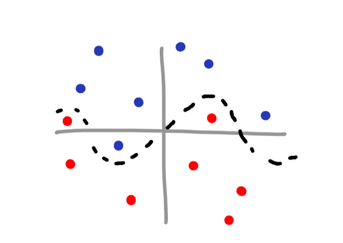
You may notice that this is a sinusoidal wave – the equation y = sin(x). Since we know the pattern of the data, it is still possible to classify the data! Though it may not be intuitive at first, all we need to do is create an additional feature to help us make the decision boundary.
features = [[x1, y1], [x2, y2], [x3, y3], ... , [xn, yn]]
for x in feature_training:
    x.append(sin(x[0]))
>> [[x1, y1, z1], [x2, y2, z2], [x3, y3, z3], ... , [xn, yn, zn]]
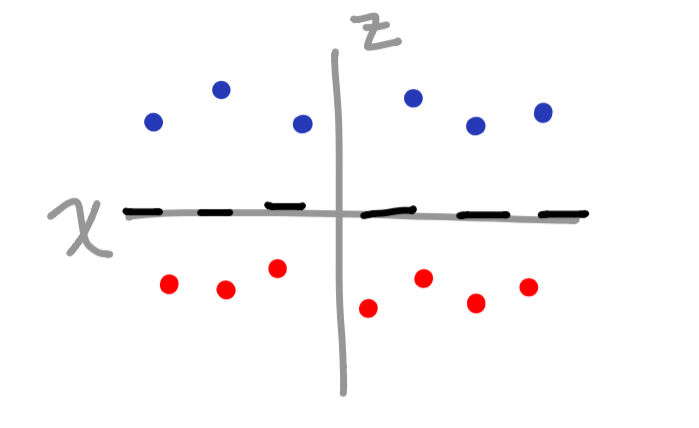
Now that we converted our vector space into a third dimension (based on the sine function), we have a clear separation of data when graphed.
The cool thing is that you can add as many features as you feel necessary to divide the vectors appropriately. The one drawback is that it can get fairly overwhelming once the data gets much more complex. So, what happens when there is a pattern that we cannot clearly define? This is where the kernel comes into play.
Kernel
There are a couple of parameters that are important to be aware of while using SVM. These parameters are also specified in the sklearn documentation. The most important one is the kernel. Also know that the kernel is not only limited to SVM, it can be used for other machine learning algorithms as well.
Imagine working with a dataset that has an extremely large set of features.
test_features = [[1, 2, 3, ... 10000], ... 100000]
Now if we had a feature containing 10,000 indicies, and we have to train on 100,000 of these inputs, you can probably imagine that this would take a really long time. Never fear, the kernel is here!
The kernel trick is very useful if you need to build a classifier given a very complex input. It is able to generalize a large amount of information without having to individually associate each feature index with a label.
There are many different types of kernel functions, and as you would imagine, each one is used in different situations. Even though Sklearn provides many different kernel functions (linear, poly, rbf, sigmoid, or precomputed), you can even make your own. Here are a few scatterplot examples as well as which kernel type should be used.
linear kernel
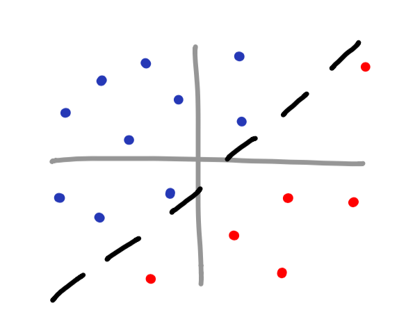
poly kernel
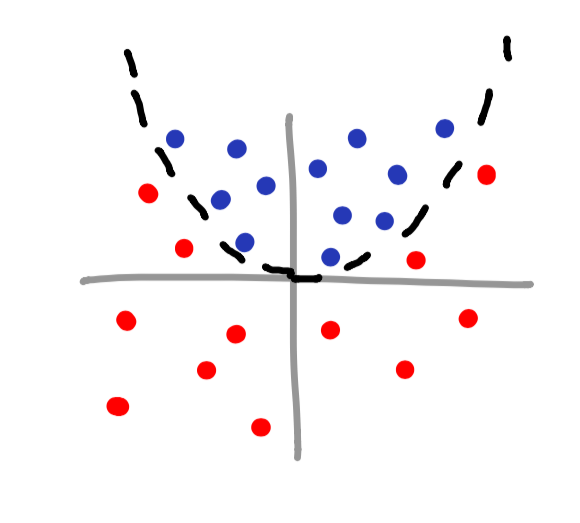
rbf kernel
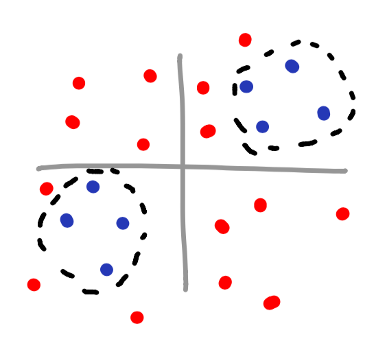
Notice how you can even make your own islands for classifying data? This is a perfect example of using a kernel to classify data that has no obvious mathematical function associated with it.
Overfitting
One issue that you may fall victim to is overfitting. Overfitting occurs when a complex function is provided for a dataset that is not as complicated. Imagine the RBF kernel was used to classify the below dataset.
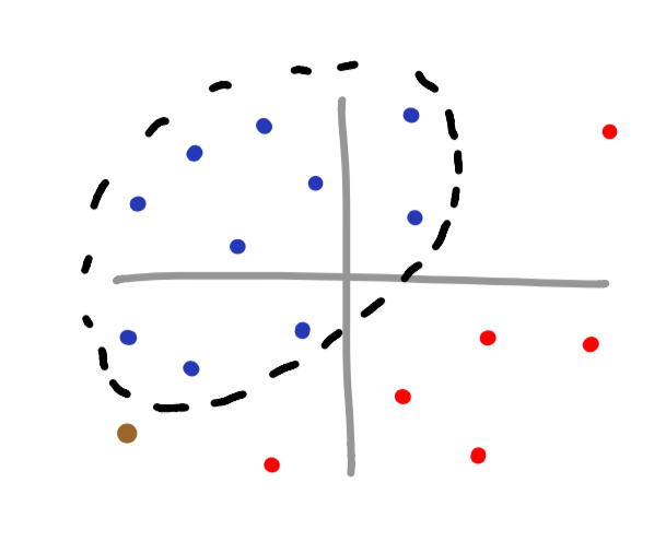
If the brown vector is supposed to be associated with the blue dataset, we can see that we have just misclassified the brown datapoint. Notice how if a linear function were to be used, we would not have misclassified this data.
Usage
Despite the differences between SVM and Naive Bayes, Sklearn uses a very similar syntax. In fact, if we wanted to express last weeks example with SVM, we could just copy/paste the code, and make some slight modifications. All we need to do is import sklearn.svm.SVC and use it the same way we used GaussianNB.
Since this is very similar to the GaussianNB, I will be implementing the SVM with pseudocode.
import numpy as np
from sklearn.svm import SVC
features = [[1, 2, 3], [4, 5, 6], ..., [x, y, z]]
labels = [0, 1, ..., 0]
classifier = SVC()
classifier.fit(features, labels)
Conclusion
All in all, SVMs are great for classifying more complicated data that does not have an intuitive pattern. However be careful, SVMs are much slower compared to other algorithms, so it may not be the best option when working with large datasets. Additionally, SVMs are not very noise tolerant, so be careful if you’re working with fuzzy datasets.
Finally, the kernel trick is wonderful for classifying data in a more generalized fashion. This not only allows us to classify datasets with an infinite number of features, but also increases performance!