Welcome to the fourth blog post in the series on machine learning. This post is a supplement of the Udacity course Intro to Machine Learning. Be sure to check out the course if you find Decision Trees interesting.

Decision Trees

Decision trees are a supervised machine learning technique to classify information. They take a dataset and break each node down into smaller subcategories. These subcategories are based on the features (characteristics) in the dataset.

Let’s start with a simple example. Suppose you want to know if you should spend time on your favorite hobby tonight. For me, one of my hobbies is coding for fun. What different factors could influence my decision? Two that come to mind are:

• The number of other chores that I still need to complete.
• The amount of coffee that I recently had.

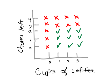
It’s reasonable that if I have at least two chores left tonight, and have had at least one cup of coffee, then I can indulge in a bit of code. As you can see, the scatterplot is fairly simplistic.

Unfortunately we cannot divide this data with a single decision boundary given the square shape. However since we are working with trees, we can make an additional boundary to classify our data.

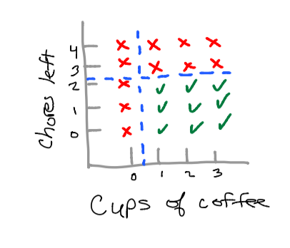
Now that we have divided our scatterplot into two categories: “yes, I can code tonight”, or “No, I cannot code tonight.” We can build a decision tree that will calculate out an output (label) for our inputs (features).

Suppose I have 1 chore left, and I have had one cup of coffee. Let’s construct a tree that will help us make a decision given the situation. X will be the cups of coffee, and Y will be the number of chores left.

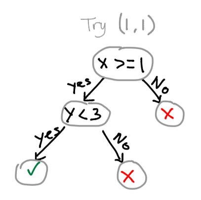
If you followed the tree correctly, you will find yourself on the lower-left leaf. This means we can code tonight!

Using the sklearn library, we can develop a code implementation:

from sklearn import tree
features = [[0, 0], [0, 1], [0, 2], [0, 3], [1, 0], [1, 1], [1, 2], [1, 3], [2, 2], [2, 3], [3, 2], [3, 3]]
labels = [0, 0, 0, 0, 1, 1, 1, 0, 1, 0, 1, 0]
clf = tree.DecisionTreeClassifier()
clf.fit(features, labels)
result = clf.predict([2, 1])
print result
>> [1]

Information Gain

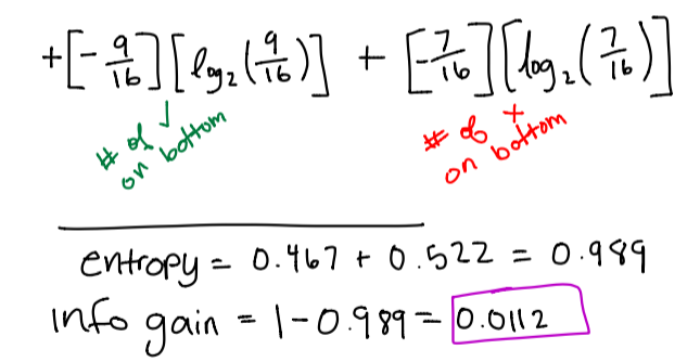
Using a metric called information gain, we can evaluate the best place to make a decision boundary. Let’s take a look at our example once again. Suppose you’re trying to determine whether the purple line or the orange line is better for dividing your data.

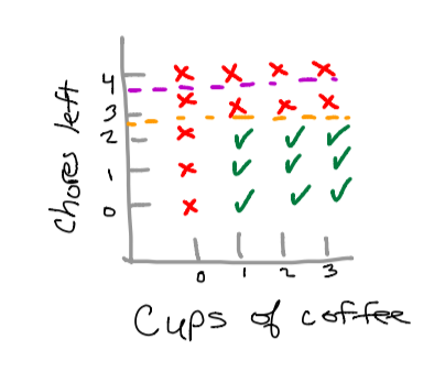
With human intuition we know that the best place to make a division is by using the orange line. So how do we evaluate this with math? We utilize the entropy equation and information gain equation to find the best outcome.

Purple calculation

Orange Calculation

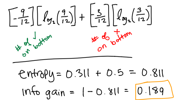
Since our information gain is greater with our orange calculation, this means we should prefer the orange decision boundary compared to the purple decision boundary.

If you have more features, you can further divide the dataset into smaller subcomponents by calculating more decision boundaries.

Conclusion

Decision Trees are a method of supervised learning that allow you to classify data based on breaking datasets into smaller components. These components are broken down based on the features in a dataset. One benefit of using Decision Trees is that you can easily visualize your data. Stay away from decision trees if you have a lot of features – this may result in overfitting your data.